The Star of Embarkation: Planet and Art
Left-drag: rotate · Right-drag: light
Map requirements and Photoshop sketches
The map needs to serve the story of The Star of Embarkation. Humans arrive on the planet and come into conflict with the native Sylphs, with both sides divided into groups supporting or opposing war. I therefore need geographic buffers between factions, rivers to supply towns, and steep mountains where a refuge can plausibly exist.
The story does not involve naval warfare, so dividing it across several main continents would change its course considerably. I kept one main continent, with a crescent-shaped opening caused by an ancient impact and a broad interior for the desert needed in the story. While drawing it, I found that a single continent felt unconvincing on its own, so I added surrounding archipelagos.
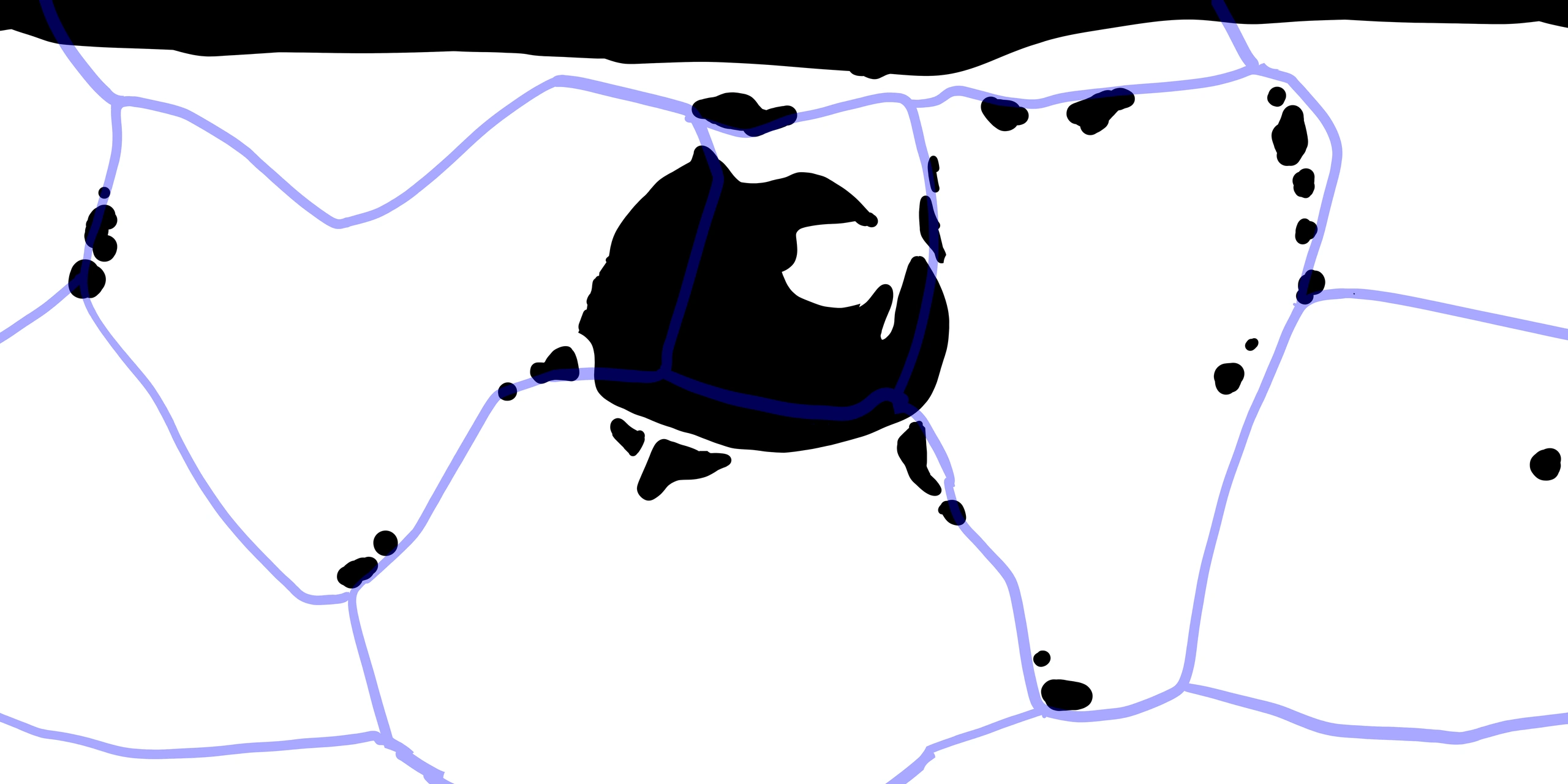
From a flat sketch to a sphere
I first sketched the continent, islands and plates in Photoshop. Outlines that looked right on a flat map became distorted on a sphere, and their apparent scale changed. To draw them in their actual spherical relationship, I switched to GPlates for the continent and plate boundaries.
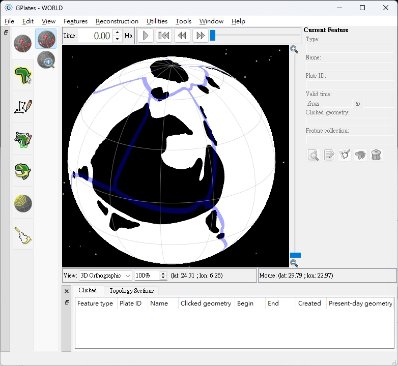
Drawing continents and plates in GPlates
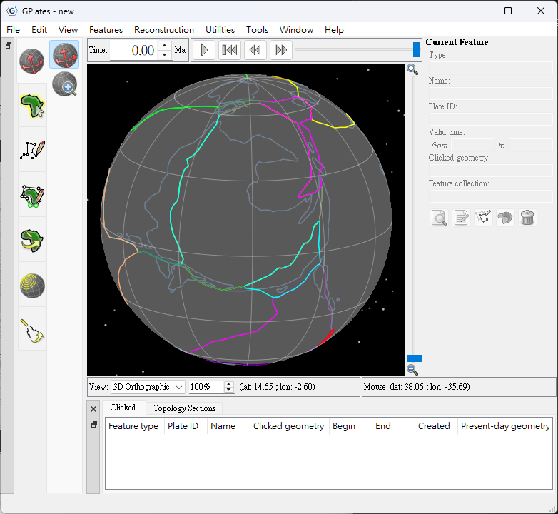
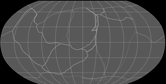
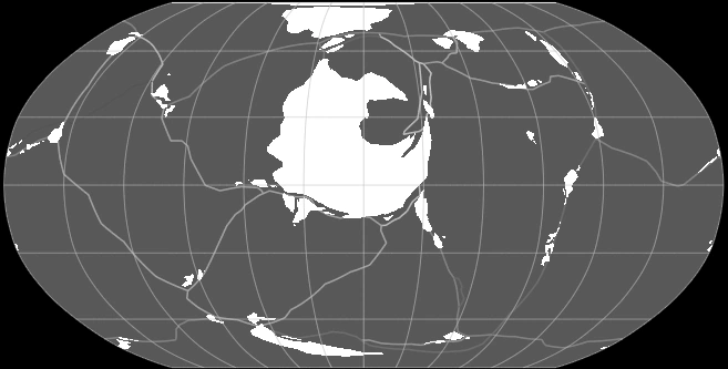
Major mountain ranges need a plausible tectonic setting, so I drew the plates before the mountains. I placed the New Andes in the west where the Newland and Westcape plates converge. The surrounding archipelagos also follow relationships between plate boundaries, subduction and smaller local plates.
In GPlates, I drew the continent as closed polygons and connected shared plate edges using topology. I set the planet's diameter to 12,050 kilometres, then checked the continental scale with the measuring tools. The main continent covers approximately 36.01 million square kilometres.
Naming geographic regions
I wanted the names to feel like real geographic names while distinguishing how humans and native Sylphs refer to the same places. Humans reached this world through The Embarkation Plan, so they call it The Star of Embarkation. The Sylphs fear fire and revere water, naming their planet Blue after the colour of water.
To humans, the continent is Newland, suggesting a new beginning. The Sylphs call it Rootland because it supports the roots of their living tree. Humans name the mountain range the New Andes after a familiar place; the Sylphs call it The Headwaters Range.
Building base terrain in QGIS
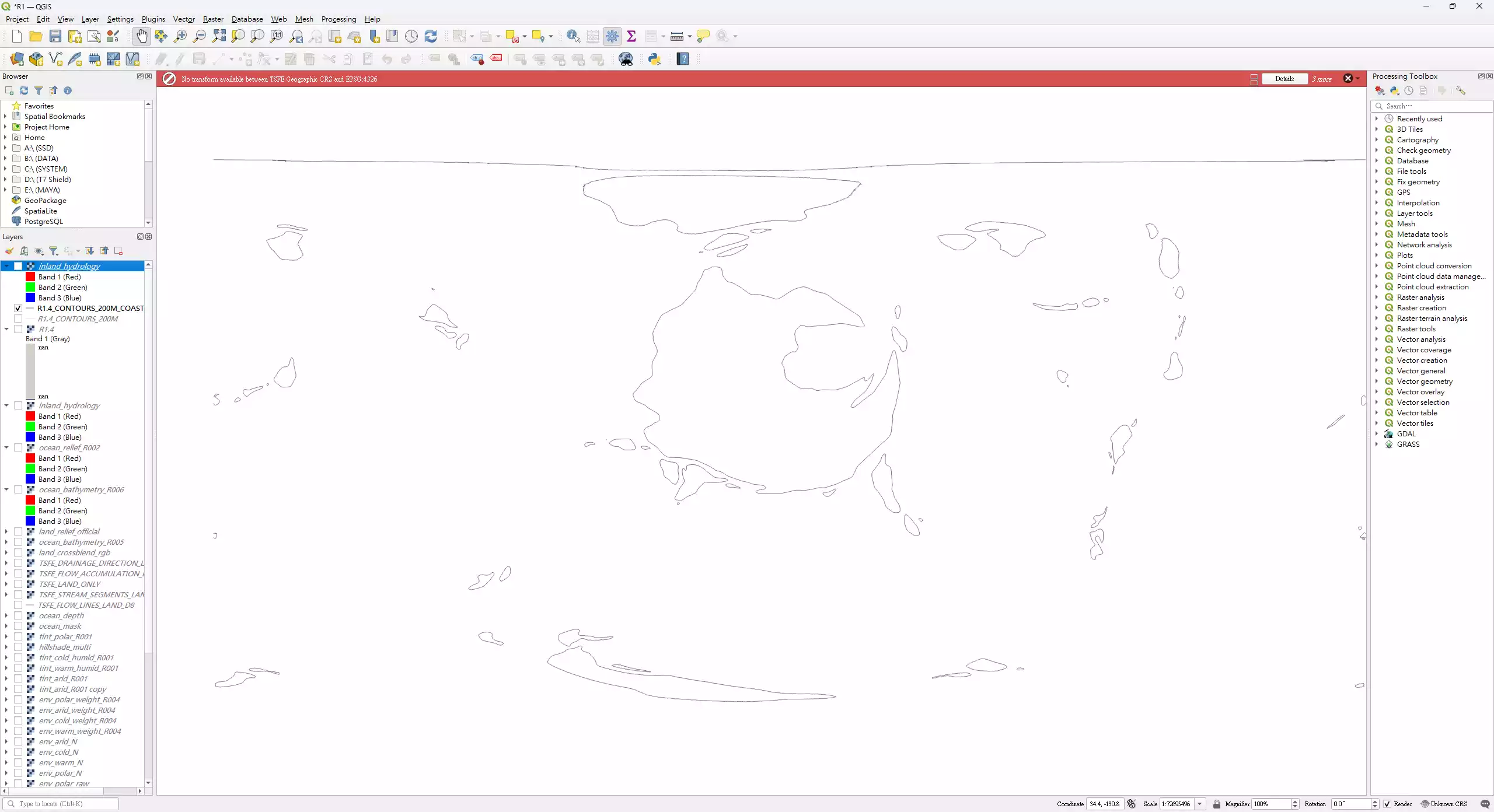
Drawing every contour by hand would require considerable work and make it difficult to think about the shape of the mountains. I drew ridge lines instead: first establishing the main ranges in QGIS, then assigning different heights to ridge nodes so the software could fill the slopes between the ridges and the coast.
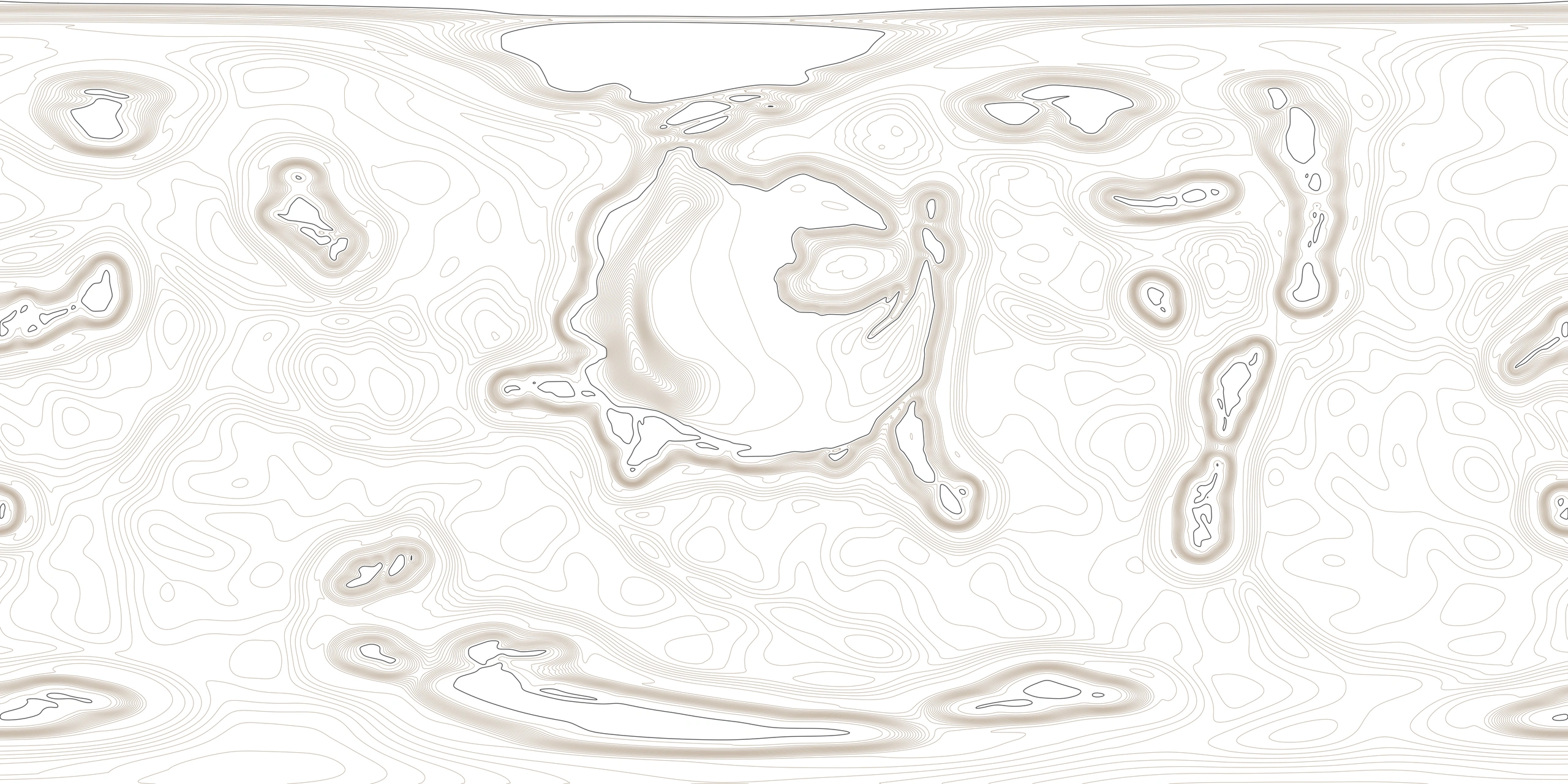
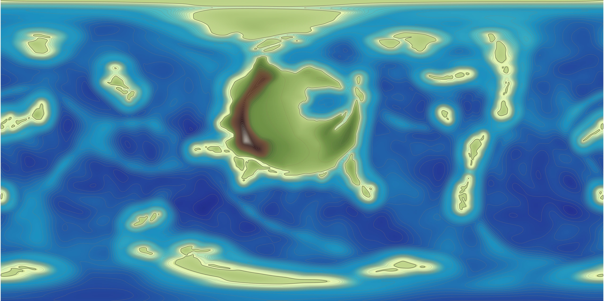
The ocean also needs terrain. I combined land and seabed in one global elevation map, using negative elevations for the sea, zero for the coast and positive elevations for land. Continental shelves, slopes and deep basins share one continuous surface, and the contour map includes the seabed.
Comparing smoothing methods
I first generated the base terrain with natural-neighbour interpolation in SAGA GIS. It estimates heights between nearby known elevations, filling the space between the ridges and the zero-elevation coast with a complete initial surface.
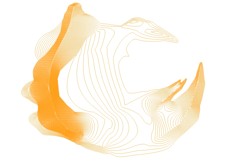
Ridge controls and a zero-elevation coast establish the base land terrain.
Smoothing was much harder than I expected. It needed to preserve the main ranges and coast while handling spherical projections and map seams. I compared two alternatives using the same ridge and coastal controls: TIN interpolation in QGIS connects known elevations into triangles and calculates heights within each triangle, but left distinct facets on the slopes; regularised splines in GRASS GIS connect the known heights with a continuous surface, but introduced seams between computational partitions.
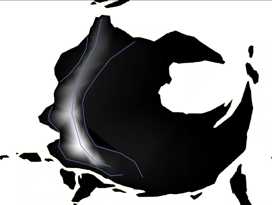
The control lines are preserved, but distinct triangular facets appear on the slopes.
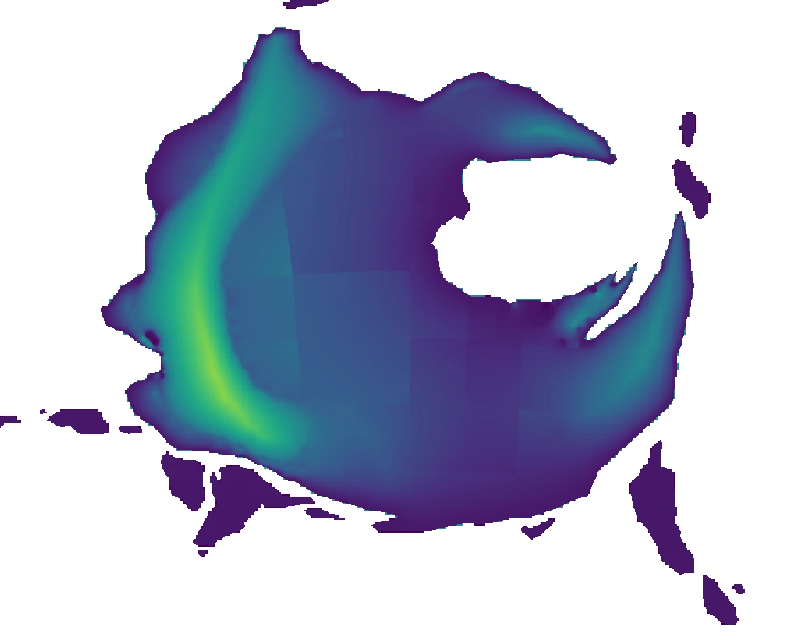
The surface is smoother, but square seams follow the computational partitions, leading me to change methods.
I settled on the natural-neighbour base terrain followed by Screened Poisson slope smoothing. This makes neighbouring slopes more consistent while constraining the surface with the original heights: the main ridges still control elevation and the coast stays at zero, giving more continuous transitions between peaks, foothills and plains.
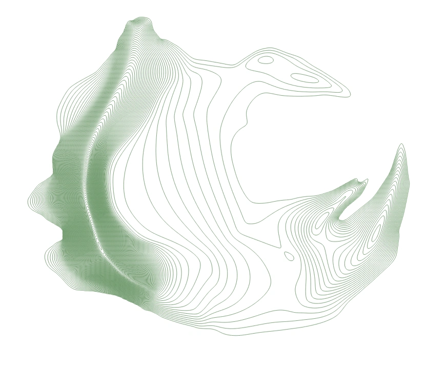
Slope smoothing connects peaks, foothills and plains while preserving the main ranges.
To reduce the cost of repeated trials, I connected these operations with Python, using GDAL to convert between local projections and global rasters, and SciPy for numerical processing. This let me compare methods using the same ridge and coastal controls.
Global elevation and contours
The resulting global elevation map measures 18,000 × 9,000. After completing the contours, I coloured the map according to their elevations to examine the overall result.
Climate simulation and terrain adjustments
Once the base terrain was ready, I needed to know where forests, deserts and rivers should occur, so I began simulating global temperature and rainfall. I also use the results to revise the terrain and check whether the continental interior, opposite mountain slopes and highlands fit the story.
Choosing the climate software
I first tried Isca, then compared GPU calculations in SpeedyWeather. SpeedyWeather was faster, but rainfall anomalies appeared in the tests, so I chose ExoPlaSim for the climate simulations.
To compare terrain and environmental settings repeatedly, I wrote scripts that run the model year by year, record global mean temperature and assess stability from its changes. I then extract temperature and rainfall from the saved results, convert them into geographic rasters, and inspect them in QGIS and SAGA GIS.
V2: Checking the terrain under Earth conditions
I first placed my terrain in an Earth reference environment to see what temperature and rainfall patterns its continent, mountains and oceans would produce. This let me inspect the terrain before gradually adding the environmental differences between Earth and The Star of Embarkation.
V2 uses T42, a model grid of 128 × 64 cells. The atmospheric model retains its Earth reference radius, gravity, pressure and irradiation, while the terrain comes from my planet map. Temperature is shown first, followed by rainfall.
ExoPlaSim · T42 (128 × 64) · Earth reference environment
Model radius 6371.22 km; gravity 9.80665 m/s²; pressure 101100 Pa.
Irradiation 1367 W/m²; model year 360 days.
ExoPlaSim · T42 (128 × 64) · Earth reference environment
Model radius 6371.22 km; gravity 9.80665 m/s²; pressure 101100 Pa.
Irradiation 1367 W/m²; model year 360 days.
V3: A smaller planet with lower gravity and pressure
In V3, I changed the model radius to 6,025 kilometres and reduced gravity and atmospheric pressure to begin testing the planet’s physical scale. I kept T42 resolution and the Earth reference irradiation.
I also kept rotation and seasonal conditions close to Earth: a configured rotation period of one Earth day, a tilt of 23.441°, and an orbital period of 365.25 Earth days. This let me examine temperature and rainfall on the smaller planet before changing its day length and seasons.
ExoPlaSim · T42 (128 × 64) · Planet-sized Earth-like conditions
Model radius 6025 km; gravity 9.022118 m/s²; pressure 92005.52 Pa.
Configured rotation period 1 Earth day; tilt 23.441°; orbital period 365.25 Earth days.
Irradiation retained at 1367 W/m².
ExoPlaSim · T42 (128 × 64) · Planet-sized Earth-like conditions
Model radius 6025 km; gravity 9.022118 m/s²; pressure 92005.52 Pa.
Configured rotation period 1 Earth day; tilt 23.441°; orbital period 365.25 Earth days.
Irradiation retained at 1367 W/m².
V4: Increasing the Earth reference resolution
V4 examines a finer model grid. I used the Earth reference environment again and increased resolution from T42 to T63, or 192 × 96 cells, to compare climate patterns around mountains, coasts and the continental interior.
This test retains the Earth reference radius, gravity, pressure and irradiation for comparison with V2. The recorded interval from configuration to completion was about 49 hours 36 minutes.
ExoPlaSim · T63 (192 × 96) · Earth reference environment
Model radius 6371.22 km; gravity 9.80665 m/s²; pressure 101100 Pa.
Irradiation 1367 W/m²; model year 360 days.
ExoPlaSim · T63 (192 × 96) · Earth reference environment
Model radius 6371.22 km; gravity 9.80665 m/s²; pressure 101100 Pa.
Irradiation 1367 W/m²; model year 360 days.
V6: Previewing the planet’s environment at lower resolution
Higher resolution quickly increased the running time, and renting server capacity was expensive. While adjusting the environmental parameters, I therefore reduced resolution to T21, or 64 × 32 cells, so each trial could produce temperature and rainfall results sooner.
V6 uses the planet’s radius, gravity and pressure, with a 20-hour solar day, an orbital period of 380 Earth days and a tilt of 16°. I first retained 100% of the Earth reference irradiation to inspect the climate under these day-length and seasonal settings. The recorded interval for this trial was about 44 minutes 20 seconds.
ExoPlaSim · T21 (64 × 32) · Planetary 16° setup
Radius 6025 km; gravity 9.022118 m/s²; pressure 93219 Pa.
Solar day 20 hours; configured orbital period 380 Earth days; tilt 16°.
Irradiation 1367 W/m² (100% of the Earth reference).
ExoPlaSim · T21 (64 × 32) · Planetary 16° setup
Radius 6025 km; gravity 9.022118 m/s²; pressure 93219 Pa.
Solar day 20 hours; configured orbital period 380 Earth days; tilt 16°.
Irradiation 1367 W/m² (100% of the Earth reference).
V7: Reducing irradiation to 99%
In V7, I retained V6’s radius, gravity, pressure, day length, orbital period and 16° tilt, while reducing irradiation from 100% to 99% of the Earth reference. I wanted to compare how this change affected temperature and rainfall.
This test also uses T21 and ran alongside the higher-resolution V5 to preview whether the temperatures suited the setting, reducing the wait and server costs. The recorded interval for this trial was about 1 hour 2 minutes.
ExoPlaSim · T21 (64 × 32) · Planetary 16° setup
Radius 6025 km; gravity 9.022118 m/s²; pressure 93219 Pa.
Solar day 20 hours; configured orbital period 380 Earth days; tilt 16°.
Irradiation 1353.33 W/m² (99% of the Earth reference).
ExoPlaSim · T21 (64 × 32) · Planetary 16° setup
Radius 6025 km; gravity 9.022118 m/s²; pressure 93219 Pa.
Solar day 20 hours; configured orbital period 380 Earth days; tilt 16°.
Irradiation 1353.33 W/m² (99% of the Earth reference).
From a wet interior to the idea of retrograde rotation
After several trials with forward rotation, I found that the continental interior was wetter than expected, and the desert needed for the story had not appeared where I intended. I had not yet understood the wind-belt directions clearly and had underestimated how moisture would travel past the mountains into the interior. This led me to revisit the relationship between rotation and winds.
To explore a drier interior, I considered retrograde rotation. I first tried a negative rotation period, but the script required a positive value. After reading about rotation and axial tilt, I then tried a tilt of about 165°. This describes how I approached the setting; the resulting climate is represented by the parameters and output saved for each run.
The climate data used in the interactive map
The interactive planet uses the same 164°, T85 dataset for temperature, rainfall and climate zones. T85 corresponds to a model grid of 256 × 128 cells. I use 15 retained years after the climate stabilised so that seasons, terrain and climate zones can be compared within one dataset.
The interval between this run’s configuration and completion records was about 6 days 4 hours 42 minutes. All durations listed here are intervals between those records and may include pauses, restarts and output processing.
Bringing climate onto finer terrain
To refine the global climate distribution around mountains, I use SAGA GIS with elevation to represent temperature differences between highlands and lowlands. For rainfall, I use GeoDS to explore moisture redistribution across mountains, accounting for wind direction, windward and leeward slopes, and elevation differences. I then compare the changes on either side of the ranges in QGIS.
Surface refinement and erosion modelling
With terrain and climate in place, I use goSPL to calculate how water affects valleys, erosion and deposition. Before that, I needed to address two issues: overly smooth mountain surfaces and a coarse climate runoff grid.
Refining overly smooth mountains
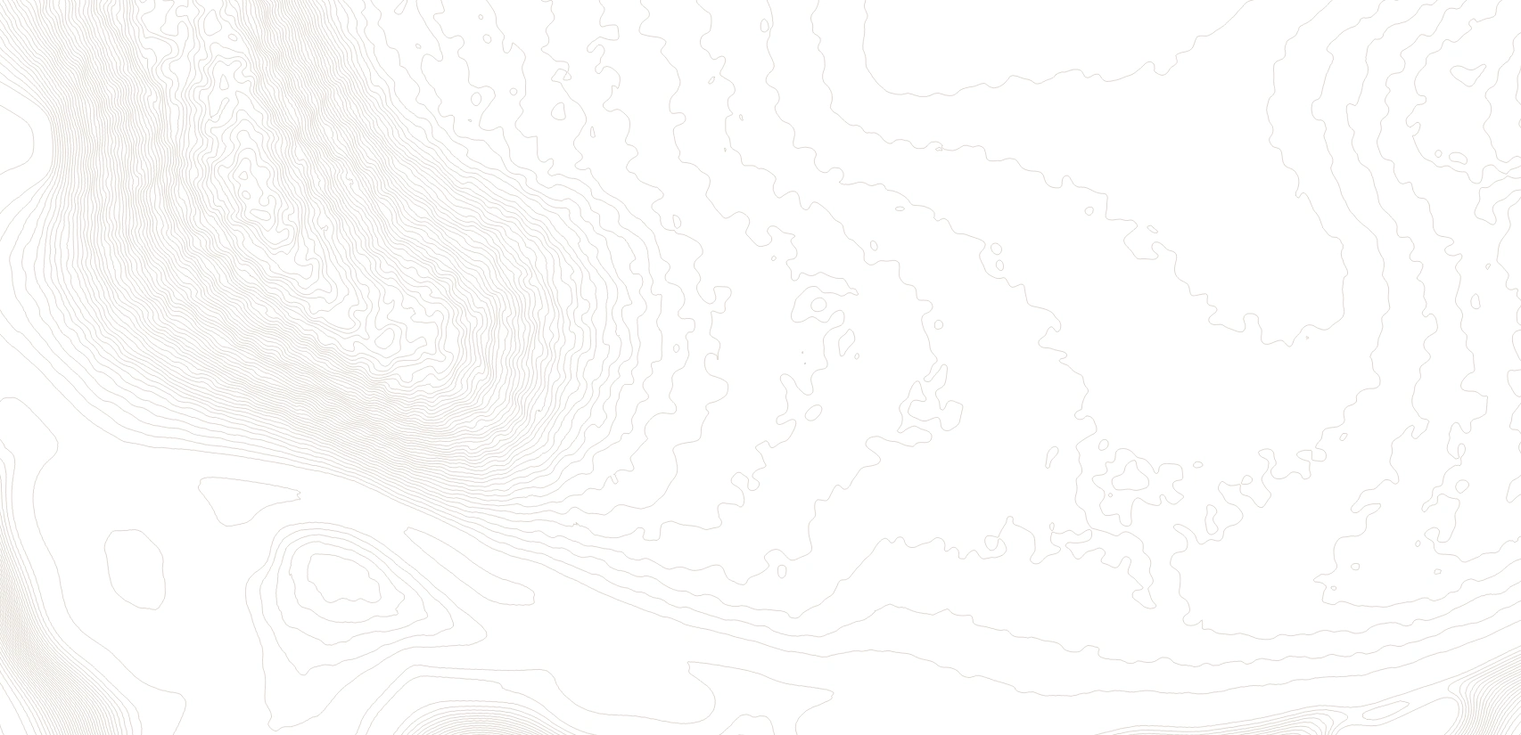
The earlier interpolation and smoothing preserved the main ranges and continental outline, but left many mountain surfaces too smooth despite their established heights. I wrote a QGIS Python tool to add continuous variations in elevation within the existing ranges.
These variations extend continuously over distances of tens of kilometres, with stronger changes at high elevations and smaller changes in lowlands. The coast and seabed stay unchanged. I then generate contours and compare the refined mountains alongside the originals.

Interpolation and smoothing establish the heights but leave an overly regular mountain surface.
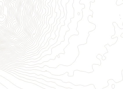
Continuous variations are added within the existing ranges; the coast and seabed stay unchanged.
The runoff refinement algorithm
The climate-model runoff pixels are coarse. Placing them directly on detailed terrain produces visible blocks, right angles and abrupt steps. I developed an interpolation method to fill continuous transitions between the original sample points and make the runoff pattern smoother.
The original sample points stay fixed and the overall total remains nearly unchanged, preserving the climate data while smoothing the transitions. The two grayscale images compare the result before and after refinement; one total-value check found a difference of approximately 0.2%.
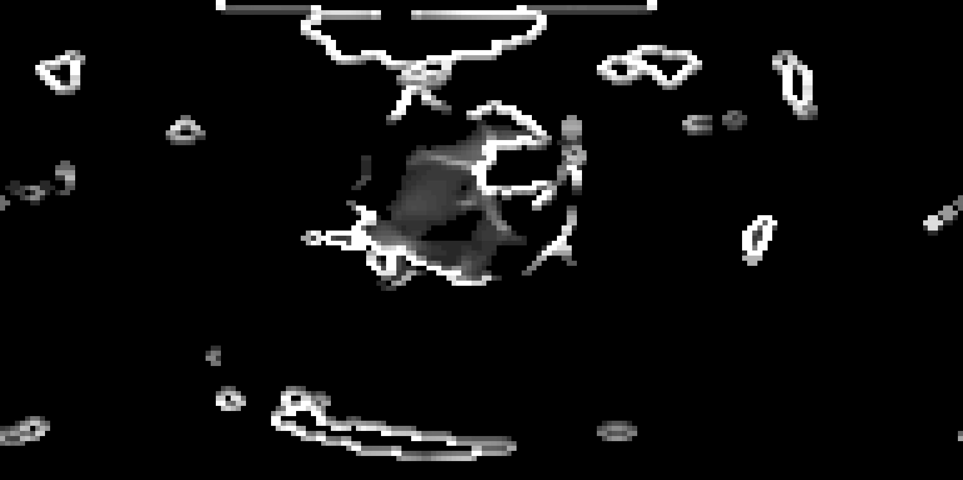
The coarse runoff grid has visible pixel boundaries.
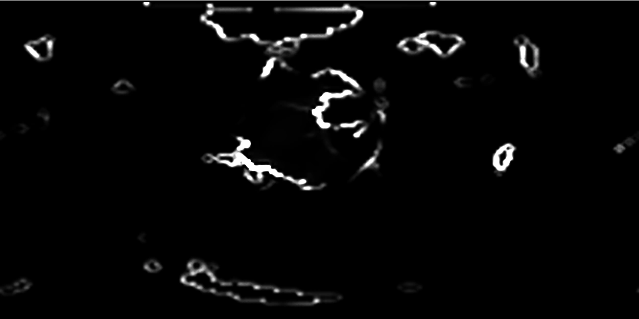
Original sample points stay fixed while continuous transitions fill the areas between them.
Calculating erosion and deposition with goSPL
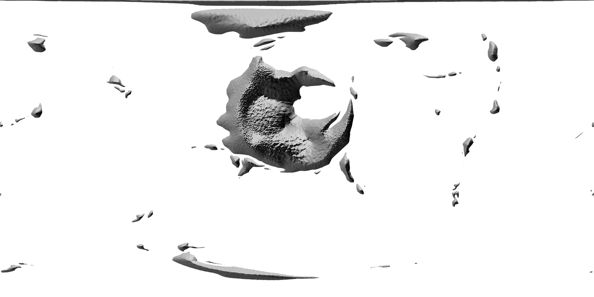
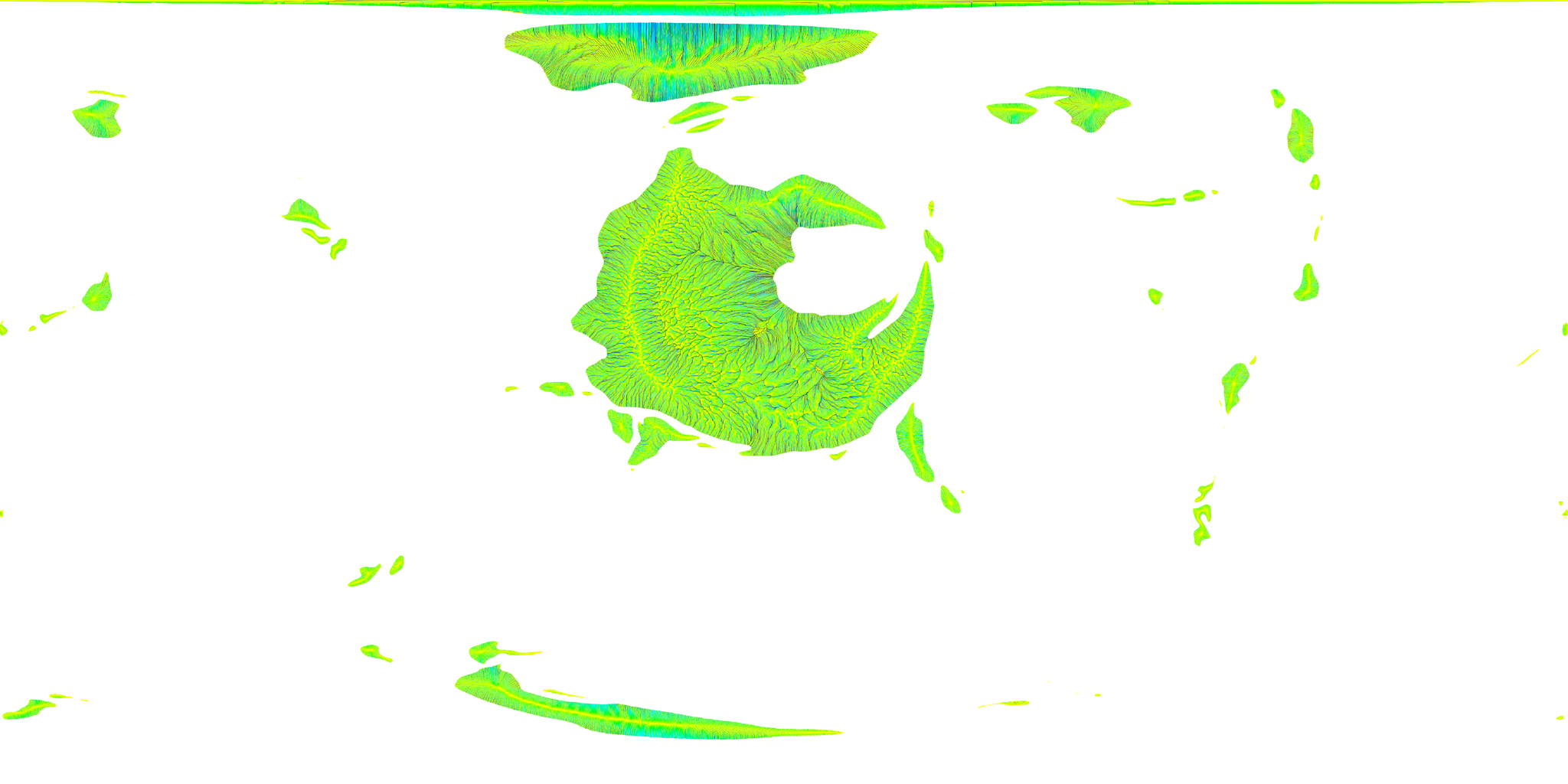
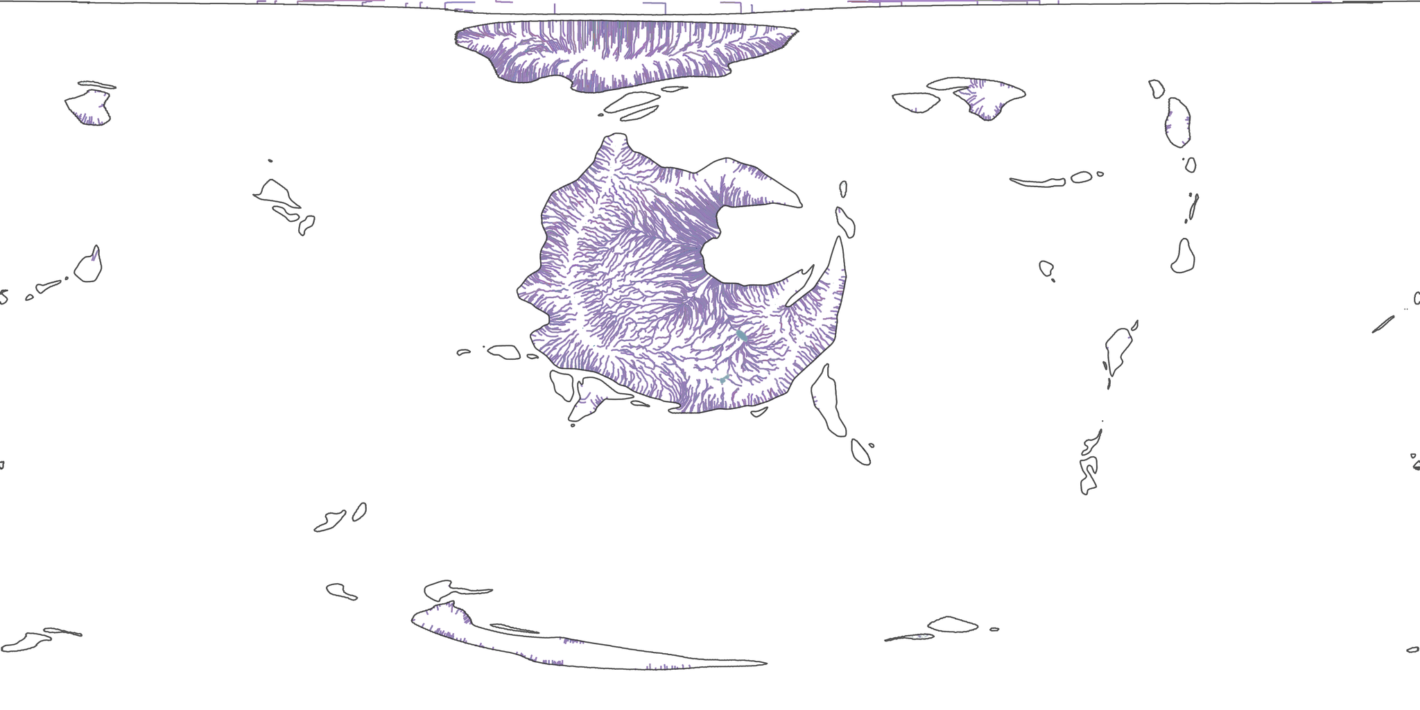
I map elevation and ExoPlaSim surface runoff onto the same spherical mesh. goSPL then calculates flow accumulation, river erosion, material transport and deposition. Water collects along lower ground and cuts into the surface, while transported material accumulates at slope bases, in valleys and across lowlands.
The program saves terrain states over simulated time. I convert these back to global geographic rasters and compare them with the original elevations and contours in QGIS, checking valley positions, mountain incision and deposition before making further map adjustments.
Planet renders and the web presentation
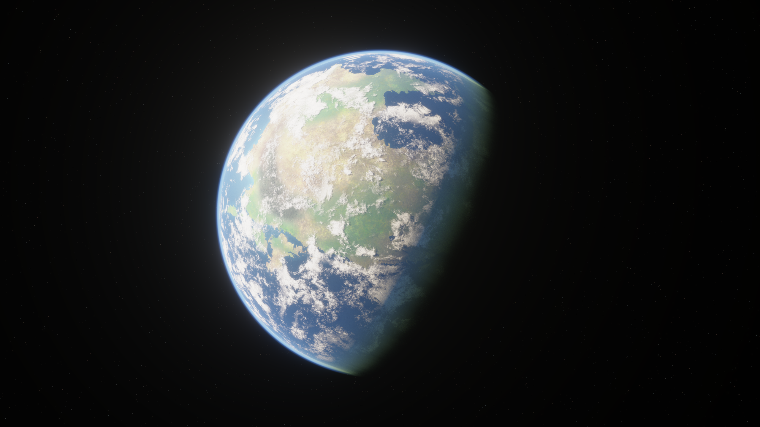
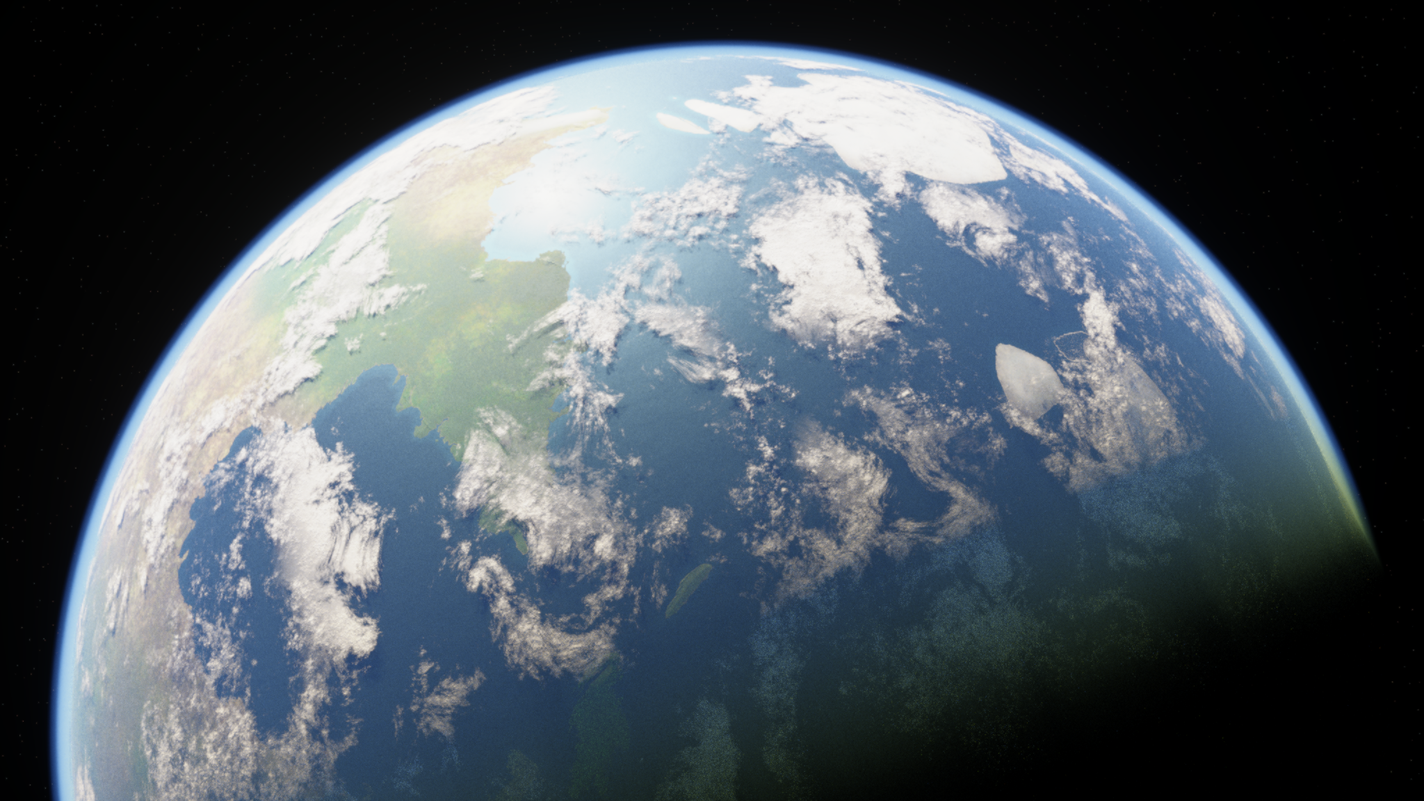
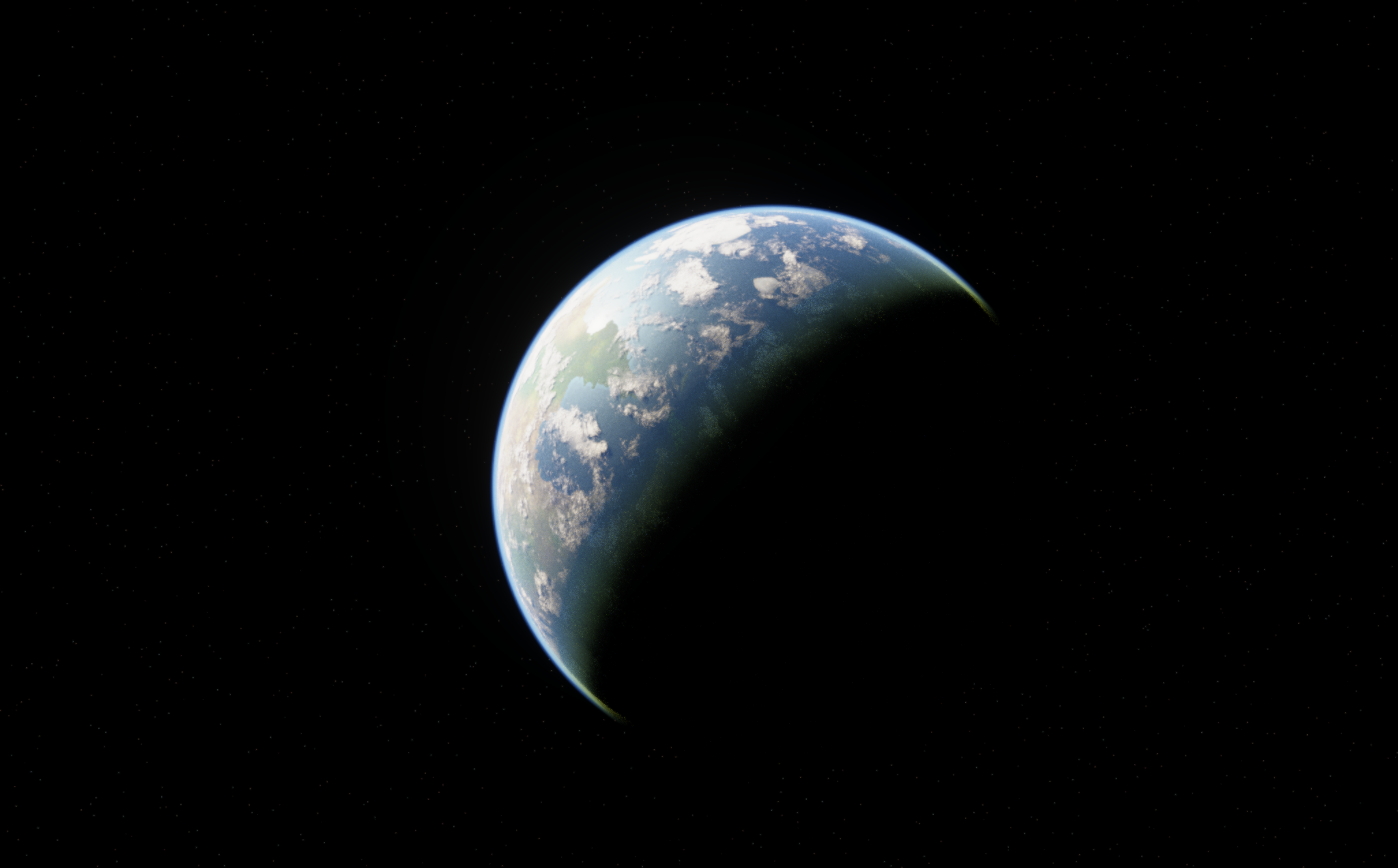
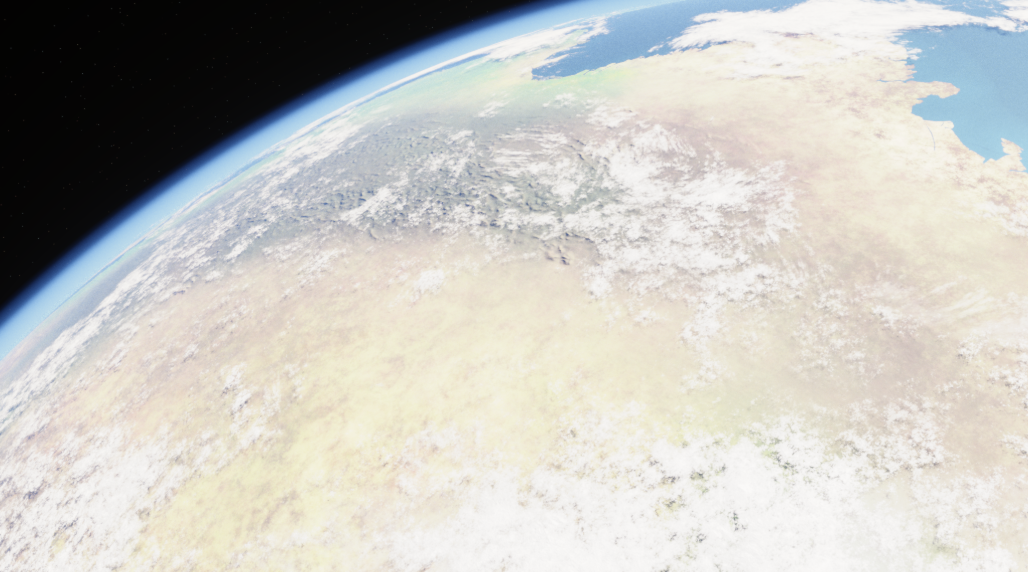
I need to see the map on the planet as a whole. In Blender, I connect my terrain and surface colours while retaining the original scene’s complex procedural cloud, ocean and atmosphere nodes. This lets me inspect mountains, coasts and climate regions together under the complete lighting, cloud shadows and atmosphere.
Final Blender Renders
The interactive planet uses Three.js. To bring the Blender surface into the browser, I export its material colours as a global UV map without baked lighting or day-and-night shadows. Normal, roughness, cloud and atmosphere data then support real-time lighting, cloud shadows and the atmosphere around the planetary limb. The illumination can respond when the planet rotates or the light moves.
Global textures contain a large amount of data, so I convert them into browser-compatible KTX2 compressed textures and retain WebP fallbacks. The surface starts with a 4,096-pixel-wide texture and loads the 8,192-pixel version for closer views. Plate, contour and climate data also load when their layers are selected, reducing the initial wait.
Coastlines, plates and contours remain vector lines. I convert their longitude and latitude into three-dimensional coordinates on a unit sphere and add intermediate points so the lines follow its surface. Positions across the ±180° longitude boundary connect as neighbours on the sphere, avoiding a vertical seam from the edges of a flat map.
To reduce the browser’s workload, the planet initialises when it enters the visible area. It redraws on demand when dragged, zoomed or switched to another layer. Seasonal playback also stops updating when the planet leaves the visible area or the page is hidden, keeping appearance, terrain and climate together for repeated comparison.